Hierarchical classifier workflow#
scpdac ships a 3-model hierarchical MLP classifier that annotates an
unlabelled PDAC dataset with fine-grained cell-type labels in a single call to
scpdac.tl.predict_labels.
The hierarchy predicts a label in two steps:
Root — a binary Malignant vs Non-Malignant classifier is applied to every cell.
Sub-classifiers — each cell is then routed, according to the root call, to either the malignant or the non-malignant fine-grained sub-classifier, which assigns the final cell type.
All three models operate on log-normalised expression (not binned counts) and automatically realign your genes to the panel they were trained on, zero-imputing any that are missing.
In this tutorial we will:
download a public PDAC dataset (Chen et al. 2025) to use as the query,
normalise it the way the classifier expects,
predict hierarchical labels, and
sanity-check the annotations on a UMAP and with canonical marker genes.
Bring your own data. The download cells below exist only for the tutorial — skip them and start from Section 2 with your own
AnnData.
Setup#
We only need the single-cell stack (scanpy, anndata), scpdac itself, and an
approximate-nearest-neighbour transformer to speed up the neighbourhood graph
used for UMAP.
import pandas as pd
import anndata as ad
import scanpy as sc
import scpdac
from sklearn_ann.kneighbors.annoy import AnnoyTransformer
1. Download the query data (tutorial only)#
We use the Chen et al. 2025
PDAC cohort (GEO accession GSE278688) — 14 samples and roughly 200,000 cells —
as an example query.
Using your own dataset? Skip straight to Section 2; none of these download cells are needed.
!mkdir /home/daniele/chen_2025
mkdir: cannot create directory ‘/home/daniele/chen_2025’: File exists
!wget "https://www.ncbi.nlm.nih.gov/geo/download/?acc=GSE278688&format=file&file=GSE278688%5Fsc%5Ffeatures%2Etsv%2Egz" -O /home/daniele/chen_2025/features.tsv.gz
!wget "https://www.ncbi.nlm.nih.gov/geo/download/?acc=GSE278688&format=file&file=GSE278688%5Fsc%5Fbarcodes%2Etsv%2Egz" -O /home/daniele/chen_2025/barcodes.tsv.gz
!wget "https://www.ncbi.nlm.nih.gov/geo/download/?acc=GSE278688&format=file&file=GSE278688%5Fsc%5Fmatrix%2Emtx%2Egz" -O /home/daniele/chen_2025/matrix.mtx.gz
!wget "https://www.ncbi.nlm.nih.gov/geo/download/?acc=GSE278688&format=file&file=GSE278688%5Fsc%5Fmetadata%2Ecsv%2Egz" -O /home/daniele/chen_2025/metadata.csv.gz
--2026-07-01 14:10:53--  https://www.ncbi.nlm.nih.gov/geo/download/?acc=GSE278688&format=file&file=GSE278688%5Fsc%5Ffeatures%2Etsv%2Egz
Resolving www.ncbi.nlm.nih.gov (www.ncbi.nlm.nih.gov)... 130.14.29.110, 2607:f220:41e:4290::110
Connecting to www.ncbi.nlm.nih.gov (www.ncbi.nlm.nih.gov)|130.14.29.110|:443... connected.
HTTP request sent, awaiting response... 200 OK
Length: 221703 (217K) [application/octet-stream]
Saving to: ‘/home/daniele/chen_2025/features.tsv.gz’

/home/daniele/chen_ 100%[===================>] 216.51K   707KB/s    in 0.3s

2026-07-01 14:10:53 (707 KB/s) - ‘/home/daniele/chen_2025/features.tsv.gz’ saved [221703/221703]

--2026-07-01 14:10:53--  https://www.ncbi.nlm.nih.gov/geo/download/?acc=GSE278688&format=file&file=GSE278688%5Fsc%5Fbarcodes%2Etsv%2Egz
Resolving www.ncbi.nlm.nih.gov (www.ncbi.nlm.nih.gov)... 130.14.29.110, 2607:f220:41e:4290::110
Connecting to www.ncbi.nlm.nih.gov (www.ncbi.nlm.nih.gov)|130.14.29.110|:443... connected.
HTTP request sent, awaiting response... 200 OK
Length: 911362 (890K) [application/octet-stream]
Saving to: ‘/home/daniele/chen_2025/barcodes.tsv.gz’

/home/daniele/chen_ 100%[===================>] 890.00K  1.50MB/s    in 0.6s

2026-07-01 14:10:54 (1.50 MB/s) - ‘/home/daniele/chen_2025/barcodes.tsv.gz’ saved [911362/911362]

--2026-07-01 14:10:55--  https://www.ncbi.nlm.nih.gov/geo/download/?acc=GSE278688&format=file&file=GSE278688%5Fsc%5Fmatrix%2Emtx%2Egz
Resolving www.ncbi.nlm.nih.gov (www.ncbi.nlm.nih.gov)... 130.14.29.110, 2607:f220:41e:4290::110
Connecting to www.ncbi.nlm.nih.gov (www.ncbi.nlm.nih.gov)|130.14.29.110|:443... connected.
HTTP request sent, awaiting response... 200 OK
Length: 1093755688 (1.0G) [application/octet-stream]
Saving to: ‘/home/daniele/chen_2025/matrix.mtx.gz’

/home/daniele/chen_ 100%[===================>]   1.02G  30.0MB/s    in 70s

2026-07-01 14:12:05 (14.9 MB/s) - ‘/home/daniele/chen_2025/matrix.mtx.gz’ saved [1093755688/1093755688]

--2026-07-01 14:12:06--  https://www.ncbi.nlm.nih.gov/geo/download/?acc=GSE278688&format=file&file=GSE278688%5Fsc%5Fmetadata%2Ecsv%2Egz
Resolving www.ncbi.nlm.nih.gov (www.ncbi.nlm.nih.gov)... 130.14.29.110, 2607:f220:41e:4290::110
Connecting to www.ncbi.nlm.nih.gov (www.ncbi.nlm.nih.gov)|130.14.29.110|:443... connected.
HTTP request sent, awaiting response... 200 OK
Length: 1166884 (1.1M) [application/octet-stream]
Saving to: ‘/home/daniele/chen_2025/metadata.csv.gz’

/home/daniele/chen_ 100%[===================>]   1.11M  1.91MB/s    in 0.6s

2026-07-01 14:12:07 (1.91 MB/s) - ‘/home/daniele/chen_2025/metadata.csv.gz’ saved [1166884/1166884]
2. Load the query dataset#
The classifier expects the query to carry raw counts. Here we read the 10x matrix, attach the published cell metadata, and stash the raw counts in a dedicated layer so later normalisation doesn’t overwrite them.
adata = sc.read_10x_mtx("/home/daniele/chen_2025")
The published metadata uses patients as the sample identifier, so we rename it
to the Sample_ID convention used throughout scpdac.
cell_metadata = pd.read_csv("/home/daniele/chen_2025/metadata.csv.gz", index_col=0)
cell_metadata = cell_metadata.rename(
    columns={
        "patients": "Sample_ID",
    }
)
adata.obs = cell_metadata
len(adata.obs.Sample_ID.unique())
14
Keep an untouched copy of the raw counts in layers["counts"] — we normalise X
in place shortly and want the originals preserved.
adata.layers["counts"] = adata.X.copy()
To keep the tutorial fast we subset the query to two patients (PA01, PA02).
In practice, run on your full cohort — the classifier scales comfortably to
hundreds of thousands of cells.
adata = adata[adata.obs.Sample_ID.isin(["PA01", "PA02"])].copy()
3. Predict hierarchical labels#
Normalise and log-transform#
The three MLPs were trained on library-size-normalised, log1p-transformed
expression, so the query must be preprocessed the same way. We normalise, take
log1p, and store the result in layers["log_norm"] — the layer we point the
classifier at below.
sc.pp.normalize_total(adata)
sc.pp.log1p(adata)
adata.layers["log_norm"] = adata.X.copy()
Run the classifier#
scpdac.tl.predict_labels loads the packaged human checkpoints, runs the root
model, routes each cell to the matching fine-grained sub-classifier, and writes
the predictions back into adata.obs — all in place. The layer argument tells
it where to find the log-normalised expression.
scpdac.tl.predict_labels(adata, species="human", layer="log_norm")
AnnData object with n_obs × n_vars = 9631 × 30543
    obs: 'tissue', 'Sample_ID', 'all_celltype', 'predicted_malignant', 'predicted_celltype'
    var: 'gene_ids', 'feature_types'
    uns: 'log1p'
    layers: 'counts', 'log_norm'
4. Inspect the predictions#
The classifier adds two columns to obs:
predicted_malignant— the root call (Malignant / Non-Malignant),predicted_celltype— the final fine-grained label.
Cross-tabulating them shows how cells are distributed across the hierarchy.
adata.obs[["predicted_malignant", "predicted_celltype"]].value_counts()
predicted_malignant  predicted_celltype
Non-Malignant        CD8+ T Cell                     4604
                     CD4+ T Cell                     1569
Malignant            Malignant Cell - Epithelial      623
Non-Malignant        Macrophage                       615
                     Cancer Associated Fibroblast     528
Malignant            Malignant Cell - Mesenchymal     411
Non-Malignant        B Cell                           332
                     NK Cell                          282
                     Endothelial Cell                 243
                     Neutrophil                       175
                     Ductal Cell (atypical)            72
                     Mast Cell                         66
                     Acinar (REG+) Cell                31
                     Plasma Cell                       19
                     Schwann Cell                      13
                     Mixed T Cell                      11
                     Ductal Cell                       11
                     Dendritic Cell                     6
                     Acinar Idling Cell                 6
Malignant            Malignant Cell - EMT               4
Non-Malignant        Monocyte                           4
                     Beta Cell                          3
                     Other Endocrine                    2
                     Pericyte                           1
Name: count, dtype: int64
Visualise on a UMAP#
To eyeball the annotations we build a standard PCA → neighbours → UMAP embedding.
The AnnoyTransformer gives an approximate but much faster neighbourhood graph.
sc.pp.pca(adata)
sc.pp.neighbors(adata, transformer=AnnoyTransformer(15))
sc.tl.umap(adata)
adata
AnnData object with n_obs × n_vars = 9631 × 30543
    obs: 'tissue', 'Sample_ID', 'all_celltype', 'predicted_malignant', 'predicted_celltype'
    var: 'gene_ids', 'feature_types'
    uns: 'log1p', 'pca', 'neighbors', 'umap', 'predicted_malignant_colors', 'predicted_celltype_colors'
    obsm: 'X_pca', 'X_umap'
    varm: 'PCs'
    layers: 'counts', 'log_norm'
    obsp: 'distances', 'connectivities'
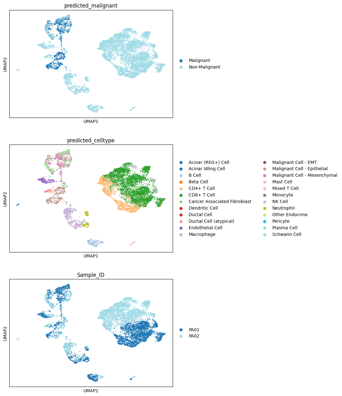
Colouring the UMAP by the predicted labels (and by Sample_ID) shows whether the
annotations form coherent, well-separated populations rather than tracking batch.
sc.pl.umap(adata, color=["predicted_malignant", "predicted_celltype", "Sample_ID"], palette="tab20", ncols=1)
Validate with canonical markers#
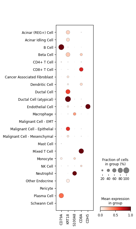
A final sanity check: canonical marker genes should light up in the expected populations — CD79A (B cells), KRT18 (epithelial / ductal), S100A8 (myeloid / neutrophils), CD8A (CD8⁺ T cells), and CDH5 (endothelium).
sc.pl.dotplot(
    adata, groupby="predicted_celltype", var_names=["CD79A", "KRT18", "S100A8", "CD8A", "CDH5"], standard_scale="var"
)