Atlas mapping workflow

Rather than a stand-alone classifier, this workflow maps a new query dataset onto a reference PDAC atlas in the atlas’s own SCANVI latent space, so query cells can be visualised and annotated side-by-side with the reference.

scpdac exposes two entry points:

• scpdac.tl.extend_atlas — performs scArches surgery on the packaged SCANVI model, fine-tuning it on your query (which may introduce entirely new batches), then returns an expanded atlas containing both reference and query cells in a shared embedding — while retaining all of your query metadata.

• scpdac.tl.embed_and_predict — the lightweight, no-surgery path: it embeds the query with the frozen reference model and transfers labels, without modifying the atlas.

In this tutorial we run both on the Chen et al. 2025 cohort and compare the resulting UMAPs.

Bring your own data. The download cells below exist only for the tutorial — skip them and start from Section 2 with your own AnnData.

Setup

We silence third-party warnings for a cleaner notebook, then import the single-cell stack, scpdac, and a fast approximate-nearest-neighbour transformer for the UMAP graph.

import warnings

warnings.filterwarnings("ignore")

import pandas as pd
import anndata as ad
import scpdac
import scanpy as sc
from sklearn_ann.kneighbors.annoy import AnnoyTransformer

1. Download the query data (tutorial only)

We use the Chen et al. 2025 PDAC cohort (GEO accession GSE278688) — 14 samples and roughly 200,000 cells — as an example query.

Using your own dataset? Skip straight to Section 2; none of these download cells are needed.

!mkdir /home/daniele/chen_2025

!wget "https://www.ncbi.nlm.nih.gov/geo/download/?acc=GSE278688&format=file&file=GSE278688%5Fsc%5Ffeatures%2Etsv%2Egz" -O /home/daniele/chen_2025/features.tsv.gz
!wget "https://www.ncbi.nlm.nih.gov/geo/download/?acc=GSE278688&format=file&file=GSE278688%5Fsc%5Fbarcodes%2Etsv%2Egz" -O /home/daniele/chen_2025/barcodes.tsv.gz
!wget "https://www.ncbi.nlm.nih.gov/geo/download/?acc=GSE278688&format=file&file=GSE278688%5Fsc%5Fmatrix%2Emtx%2Egz" -O /home/daniele/chen_2025/matrix.mtx.gz
!wget "https://www.ncbi.nlm.nih.gov/geo/download/?acc=GSE278688&format=file&file=GSE278688%5Fsc%5Fmetadata%2Ecsv%2Egz" -O /home/daniele/chen_2025/metadata.csv.gz

--2026-06-30 10:07:51--  https://www.ncbi.nlm.nih.gov/geo/download/?acc=GSE278688&format=file&file=GSE278688%5Fsc%5Fmetadata%2Ecsv%2Egz
Resolving www.ncbi.nlm.nih.gov (www.ncbi.nlm.nih.gov)... 130.14.29.110, 2607:f220:41e:4290::110
Connecting to www.ncbi.nlm.nih.gov (www.ncbi.nlm.nih.gov)|130.14.29.110|:443... connected.
HTTP request sent, awaiting response... 200 OK
Length: 1166884 (1.1M) [application/octet-stream]
Saving to: ‘/home/daniele/chen_2025/metadata.csv.gz’

/home/daniele/chen_ 100%[===================>]   1.11M  1.44MB/s    in 0.8s    

2026-06-30 10:07:52 (1.44 MB/s) - ‘/home/daniele/chen_2025/metadata.csv.gz’ saved [1166884/1166884]

2. Load the query and the reference atlas

The query needs raw counts and a Sample_ID batch column. We also load a (subsampled) reference atlas to map onto — any atlas stored as zarr/h5ad with matching raw counts works.

query = sc.read_10x_mtx("/home/daniele/chen_2025")

The published metadata uses patients as the sample identifier, so we rename it to the Sample_ID convention used throughout scpdac.

cell_metadata = pd.read_csv("/home/daniele/chen_2025/metadata.csv.gz", index_col=0)

cell_metadata = cell_metadata.rename(
    columns={
        "patients": "Sample_ID",
    }
)

query.obs = cell_metadata
len(query.obs.Sample_ID.unique())

14

Keep an untouched copy of the raw counts in layers["counts"] for the model to bin and embed.

query.layers["counts"] = query.X.copy()

For a fast demo we restrict the query to two patients and map onto a 100k-cell subsample of the human atlas. Use the full atlas and query for production runs.

query = query[query.obs.Sample_ID.isin(["PA01", "PA02"])].copy()

atlas = ad.read_zarr("/data/Daniele/atlases/final_versions/Human_subsampled.zarr")

query, atlas

(AnnData object with n_obs × n_vars = 9631 × 30543
     obs: 'tissue', 'Sample_ID', 'all_celltype'
     var: 'gene_ids', 'feature_types'
     layers: 'counts',
 AnnData object with n_obs × n_vars = 100000 × 39041
     obs: 'Sample_ID', 'Condition', 'Treatment', 'TreatmentType', 'TreatmentStatus', 'Tissue', 'Sex', 'Dataset', 'Technology', 'Level_1', 'Level_2', 'Level_3', 'Level_4', 'Age', 'Diabetes', 'Is_Core', 'EMT category', 'Dataset_ID', 'Cluster_Names'
     var: 'n_cells', 'ensembl_id', 'start', 'end', 'chromosome', 'gene_name_adata_sc', 'highly_variable_adata_sc', 'means_adata_sc', 'dispersions_adata_sc', 'dispersions_norm_adata_sc', 'highly_variable_nbatches_adata_sc', 'highly_variable_intersection_adata_sc', 'n_cells_by_counts_adata_sc', 'mean_counts_adata_sc', 'log1p_mean_counts_adata_sc', 'pct_dropout_by_counts_adata_sc', 'total_counts_adata_sc', 'log1p_total_counts_adata_sc', 'mito_adata_sc', 'n_cells_by_counts_adata_sn', 'mean_counts_adata_sn', 'log1p_mean_counts_adata_sn', 'pct_dropout_by_counts_adata_sn', 'total_counts_adata_sn', 'log1p_total_counts_adata_sn', 'Manual_Genes', 'mt', 'ribo', 'hb'
     uns: 'Condition_colors', 'Is_Core_colors', 'Level_1_colors', 'Level_2_colors', 'Level_3_colors', 'Level_4_All_colors', 'Level_4_Final_colors', 'Level_4_colors', 'UMAP_0.75', 'UMAP_0.85', '_scvi_manager_uuid', '_scvi_uuid', 'neighbors', 'umap'
     obsm: 'EMT score', 'EMT_score_DL', 'Global_Leiden', 'MALAT1_lognorm', 'UMAP_0.75', 'UMAP_0.85', 'UMAP_0.95', 'X_pca', 'X_umap', '_scvi_batch', '_scvi_labels', 'batch', 'bin_edges', 'cnv_score_abs', 'empty_droplet', 'infercnv_score_malignant', 'infercnv_score_malignant_refined', 'is_outlier_total_counts', 'leiden', 'leiden_0.2', 'leiden_0.2_annotation', 'leiden_0.5', 'leiden_subcluster', 'level0_leiden_subcluster', 'log1p_n_genes_by_counts', 'log1p_total_counts', 'log1p_total_counts_mito', 'log_counts', 'mt_frac', 'n_counts', 'n_genes', 'n_genes_by_counts', 'outlier', 'pct_counts_mito', 'scANVI_cross_species', 'scANVI_emb_final', 'scanvi_L4_emb', 'scanvi_extended_atlas_emb', 'total_counts', 'total_counts_mito'
     layers: 'counts', 'log_norm', 'raw'
     obsp: 'connectivities', 'distances')

3. Expand the atlas with scArches surgery

scpdac.tl.extend_atlas fine-tunes the packaged SCANVI model on the query (max_epochs controls the surgery length), embeds both atlas and query into the shared latent space, and concatenates them into a single expanded AnnData. The result carries a source column (atlas / query), predicted labels in predicted_celltype, and every original query obs column.

expanded = scpdac.tl.extend_atlas(query, atlas, species="human", max_epochs=10)

INFO     File /home/daniele/Code/github_synced/scPDAC/src/scpdac/models/scanvi/human_scanvi/model.pt already       
         downloaded                                                                                                
INFO     Training for 10 epochs.
Epoch 10/10: 100%|██████████| 10/10 [00:08<00:00,  1.30it/s, v_num=1, train_loss_step=1.78e+3, train_loss_epoch=1.86e+3]
Epoch 10/10: 100%|██████████| 10/10 [00:08<00:00,  1.24it/s, v_num=1, train_loss_step=1.78e+3, train_loss_epoch=1.86e+3]

expanded

AnnData object with n_obs × n_vars = 109631 × 29305
    obs: 'Sample_ID', 'Condition', 'Treatment', 'TreatmentType', 'TreatmentStatus', 'Tissue', 'Sex', 'Dataset', 'Technology', 'Level_1', 'Level_2', 'Level_3', 'Level_4', 'Age', 'Diabetes', 'Is_Core', 'EMT category', 'Dataset_ID', 'Cluster_Names', 'source', 'predicted_celltype'
    var: 'n_cells', 'ensembl_id', 'start', 'end', 'chromosome', 'gene_name_adata_sc', 'highly_variable_adata_sc', 'means_adata_sc', 'dispersions_adata_sc', 'dispersions_norm_adata_sc', 'highly_variable_nbatches_adata_sc', 'highly_variable_intersection_adata_sc', 'n_cells_by_counts_adata_sc', 'mean_counts_adata_sc', 'log1p_mean_counts_adata_sc', 'pct_dropout_by_counts_adata_sc', 'total_counts_adata_sc', 'log1p_total_counts_adata_sc', 'mito_adata_sc', 'n_cells_by_counts_adata_sn', 'mean_counts_adata_sn', 'log1p_mean_counts_adata_sn', 'pct_dropout_by_counts_adata_sn', 'total_counts_adata_sn', 'log1p_total_counts_adata_sn', 'Manual_Genes', 'mt', 'ribo', 'hb', 'gene_ids', 'feature_types'
    obsm: 'X_scANVI_emb'
    layers: 'counts'

Visualise the expanded atlas

We build a joint UMAP directly from the shared X_scANVI_emb embedding — no PCA needed, since the SCANVI latent space is already the integrated representation.

sc.pp.neighbors(expanded, use_rep="X_scANVI_emb", transformer=AnnoyTransformer(15))

sc.tl.umap(
    expanded,
)

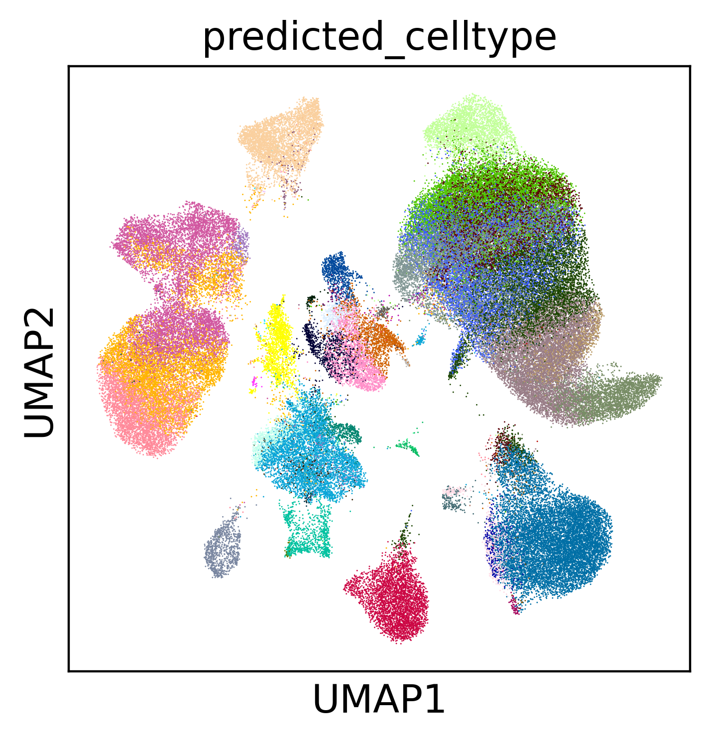
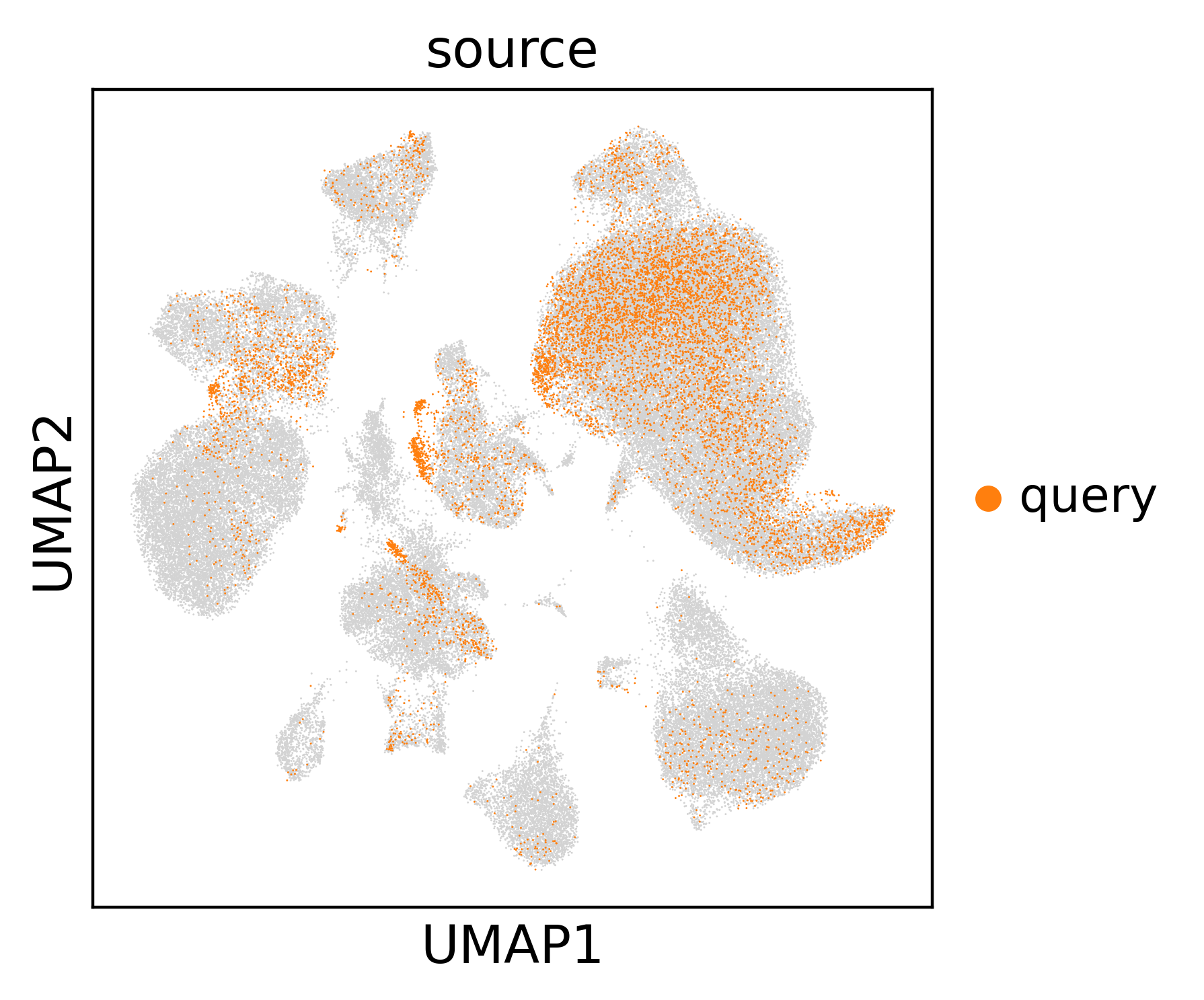
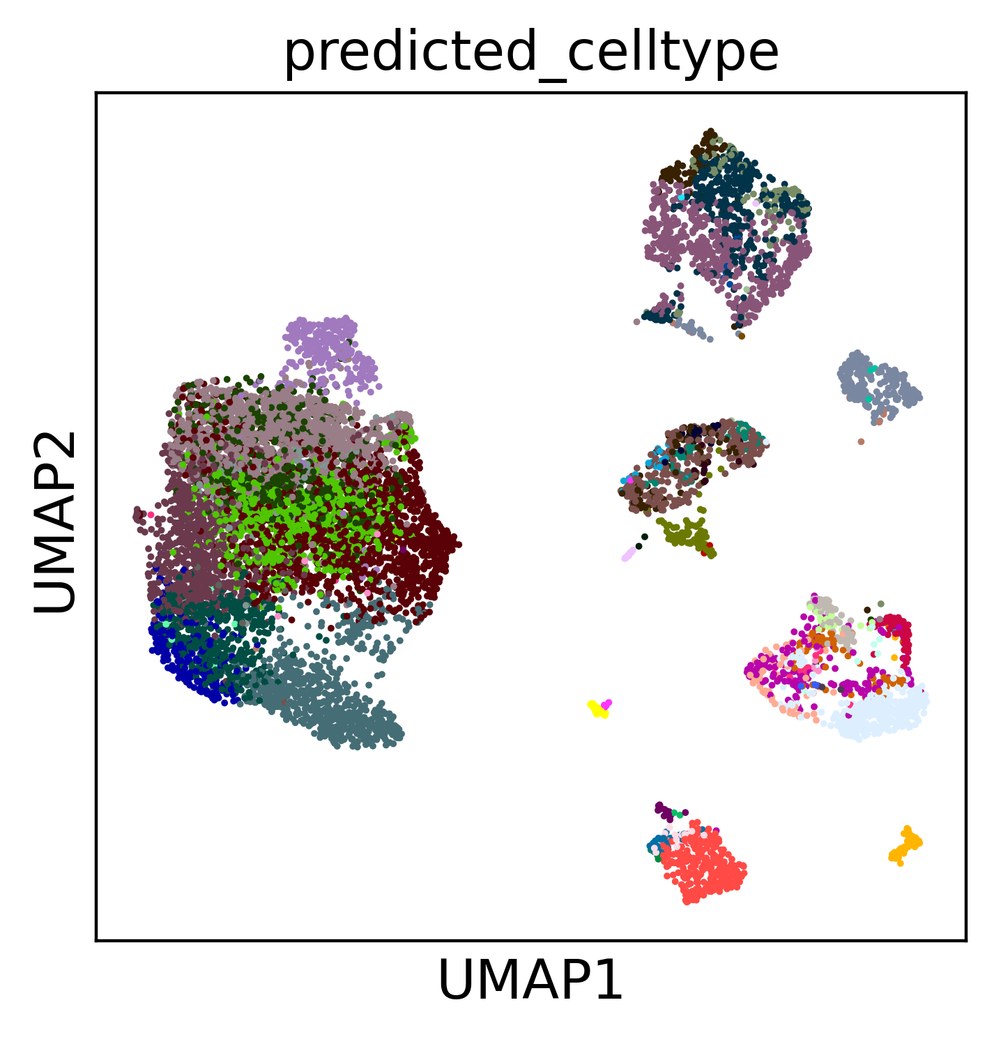
Colouring by predicted_celltype shows the transferred annotations across the combined embedding; highlighting source == "query" shows where the new cells land relative to the reference. Well-integrated query cells intermix with matching reference populations rather than forming isolated islands.

sc.pl.umap(
    expanded,
    color="predicted_celltype",
    legend_loc=None
)

sc.pl.umap(expanded, color="source", groups="query", na_in_legend=False)

expanded

AnnData object with n_obs × n_vars = 109631 × 29305
    obs: 'Sample_ID', 'Condition', 'Treatment', 'TreatmentType', 'TreatmentStatus', 'Tissue', 'Sex', 'Dataset', 'Technology', 'Level_1', 'Level_2', 'Level_3', 'Level_4', 'Age', 'Diabetes', 'Is_Core', 'EMT category', 'Dataset_ID', 'Cluster_Names', 'source', 'predicted_celltype'
    var: 'n_cells', 'ensembl_id', 'start', 'end', 'chromosome', 'gene_name_adata_sc', 'highly_variable_adata_sc', 'means_adata_sc', 'dispersions_adata_sc', 'dispersions_norm_adata_sc', 'highly_variable_nbatches_adata_sc', 'highly_variable_intersection_adata_sc', 'n_cells_by_counts_adata_sc', 'mean_counts_adata_sc', 'log1p_mean_counts_adata_sc', 'pct_dropout_by_counts_adata_sc', 'total_counts_adata_sc', 'log1p_total_counts_adata_sc', 'mito_adata_sc', 'n_cells_by_counts_adata_sn', 'mean_counts_adata_sn', 'log1p_mean_counts_adata_sn', 'pct_dropout_by_counts_adata_sn', 'total_counts_adata_sn', 'log1p_total_counts_adata_sn', 'Manual_Genes', 'mt', 'ribo', 'hb', 'gene_ids', 'feature_types'
    uns: 'neighbors', 'umap', 'predicted_celltype_colors', 'source_colors'
    obsm: 'X_scANVI_emb', 'X_umap'
    layers: 'counts'
    obsp: 'distances', 'connectivities'

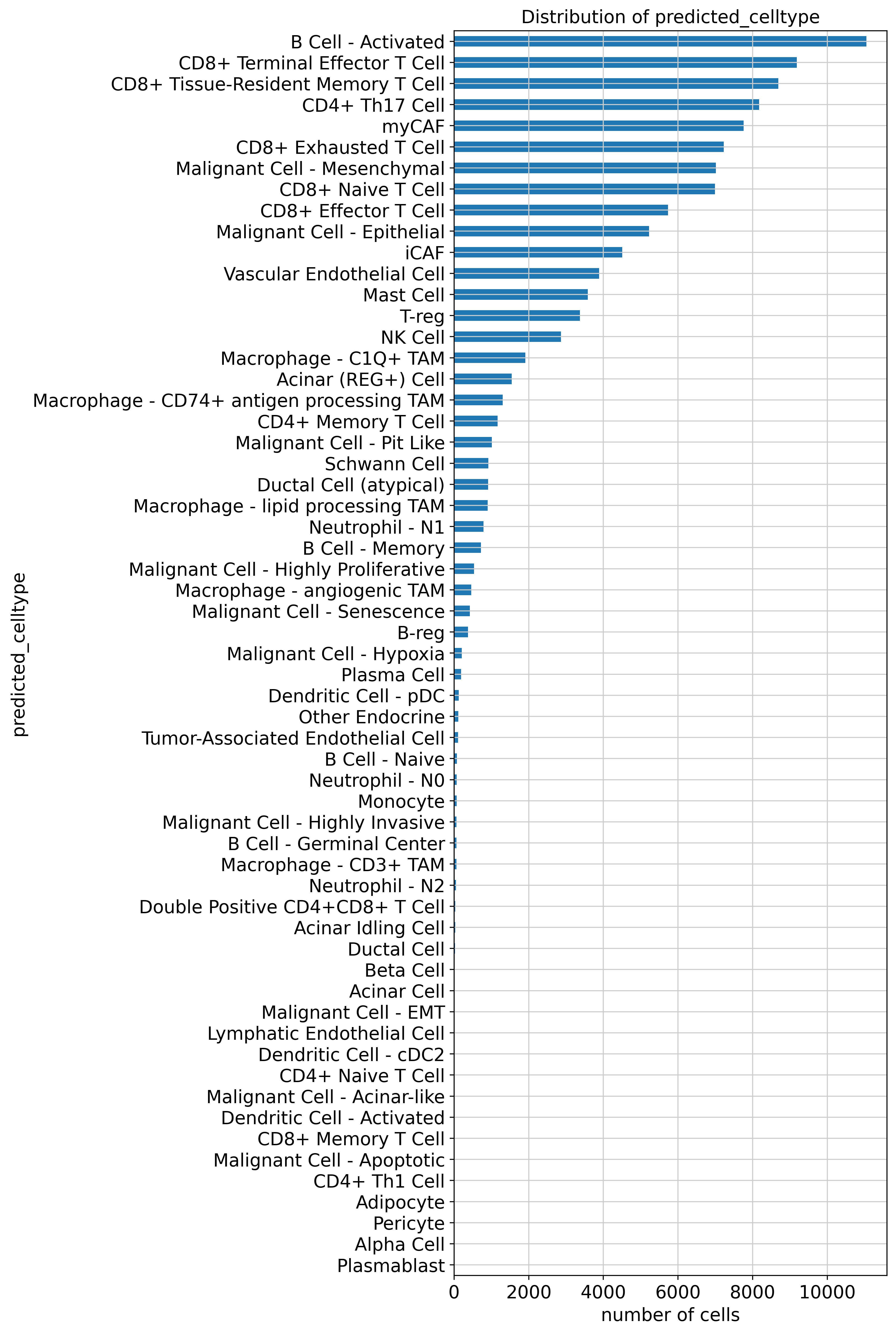
scpdac.pl.plot_label_distribution(expanded, key="predicted_celltype")

<Axes: title={'center': 'Distribution of predicted_celltype'}, xlabel='number of cells', ylabel='predicted_celltype'>

4. Embed-only: transfer labels without surgery

If you do not want to compare your data against the rest of the atlas, you can simply use scpdac.tl.embed_and_predict which embeds the query with the frozen model and transfers labels in one step — faster, and it leaves the atlas untouched. It writes the latent embedding to obsm["X_scANVI_emb"] and predictions to obs["predicted_celltype"].

query = scpdac.tl.embed_and_predict(query, "human")

INFO     File /home/daniele/Code/github_synced/scPDAC/src/scpdac/models/scanvi/human_scanvi/model.pt already       
         downloaded

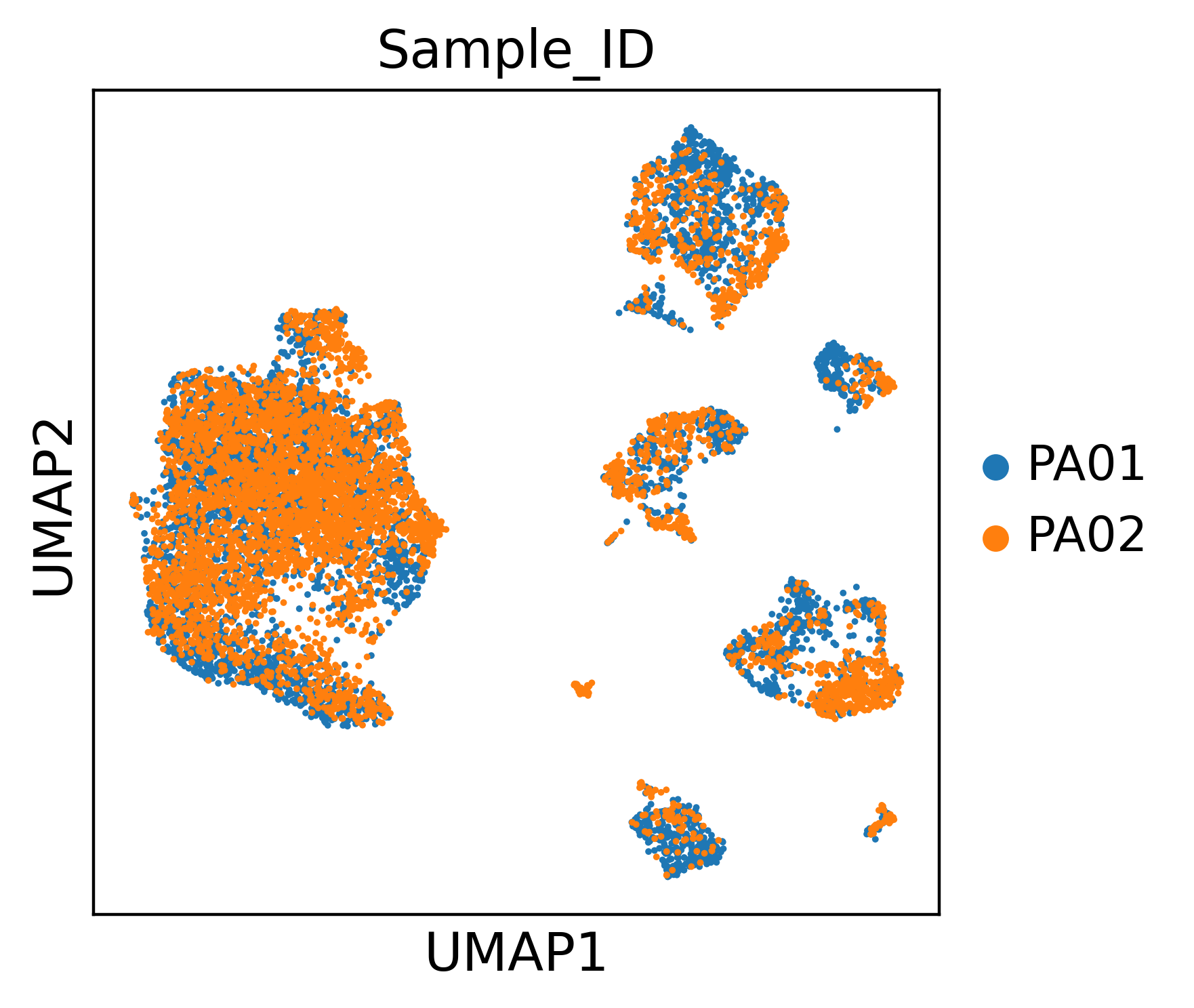
Again we compute a UMAP from the embedding and colour by the predicted cell types and by sample, to confirm the query integrates cleanly on its own.

sc.pp.neighbors(query, use_rep="X_scANVI_emb", transformer=AnnoyTransformer(15))

sc.tl.umap(
    query,
)

sc.pl.umap(
    query,
    color="predicted_celltype",
    legend_loc=None
)

sc.pl.umap(
    query,
    color="Sample_ID",
)